Quantitative Analysis#
This Jupyter notebook provides a comprehensive exploratory data analysis (EDA) of the Boston Housing dataset. It walks through data loading, cleaning, indexing, grouping, and summary statistics, with clear examples and commentary. The goal is to help users develop familiarity with pandas, numpy, matplotlib, and seaborn for quantitative analysis. Special attention is given to understanding data distribution, variable relationships, and insights related to housing near the Charles River.
Installing Libraries#
%pip install numpy
%pip install pandas
%pip install seaborn
%pip install matplotlib
import numpy as np
import pandas as pd
import seaborn as sns
import matplotlib.pyplot as plt
Exploratory Data Analysis#
Using set_option in pandas so that floating-point numbers (decimals) are shown with only 2 digits after the decimal point when printed. It helps make data tables easier to read.
For more arguments set_option can take checkout Pandas Documentation on set_options
# Set pandas options for better display of floating point numbers
pd.set_option("display.precision", 2)
Using read_csv to load a CSV file named "Boston.csv" into a pandas DataFrame called df. The using head() to display the first 5 rows, by default. We could also use head(10) if we wanted to display the first 10 rows.
Here is the data we used but, if you have data you would rather use, feel free to use it. Just make sure to change the path in the data variable.
# Load the Boston housing dataset
df = pd.read_csv("./Boston.csv")
# Display the first few rows of the dataset
df.head()
| Unnamed: 0 | crim | zn | indus | chas | nox | rm | age | dis | rad | tax | ptratio | black | lstat | medv | |
|---|---|---|---|---|---|---|---|---|---|---|---|---|---|---|---|
| 0 | 1 | 6.32e-03 | 18.0 | 2.31 | 0 | 0.54 | 6.58 | 65.2 | 4.09 | 1 | 296 | 15.3 | 396.90 | 4.98 | 24.0 |
| 1 | 2 | 2.73e-02 | 0.0 | 7.07 | 0 | 0.47 | 6.42 | 78.9 | 4.97 | 2 | 242 | 17.8 | 396.90 | 9.14 | 21.6 |
| 2 | 3 | 2.73e-02 | 0.0 | 7.07 | 0 | 0.47 | 7.18 | 61.1 | 4.97 | 2 | 242 | 17.8 | 392.83 | 4.03 | 34.7 |
| 3 | 4 | 3.24e-02 | 0.0 | 2.18 | 0 | 0.46 | 7.00 | 45.8 | 6.06 | 3 | 222 | 18.7 | 394.63 | 2.94 | 33.4 |
| 4 | 5 | 6.91e-02 | 0.0 | 2.18 | 0 | 0.46 | 7.15 | 54.2 | 6.06 | 3 | 222 | 18.7 | 396.90 | 5.33 | 36.2 |
drop() removes the column named ‘Unnamed: 0’ from the DataFrame df in place (without creating a new DataFrame). axis=1 means you’re dropping a column (not a row). inplace=True means the change is made directly to df — no need to reassign it.
# Drop the 'Unnamed: 0' column
df.drop(columns=['Unnamed: 0'], axis=1, inplace=True)
Printing DataFrames#
Displays the number of rows and columns in the dataset df. .shape returns a tuple: (num_rows, num_columns).
# Display the number of rows and columns in the dataset
print(df.shape)
(506, 14)
Prints the column names of the DataFrame df. .columns returns an Index object containing all column labels. This helps you quickly see what features (columns) are included in the dataset.
# Display the column names of the dataset
print(df.columns)
Index(['crim', 'zn', 'indus', 'chas', 'nox', 'rm', 'age', 'dis', 'rad', 'tax',
       'ptratio', 'black', 'lstat', 'medv'],
      dtype='object')
.info displays a summary of the dataset, including: number of rows and columns, column names, number of non-null (non-missing) values in each column, column data types, and memory usage. This is helpful to see if the data has any missing values.
# Display the summary information of the dataset
print(df.info())
<class 'pandas.core.frame.DataFrame'>
RangeIndex: 506 entries, 0 to 505
Data columns (total 14 columns):
 #   Column   Non-Null Count  Dtype
---  ------   --------------  -----
 0   crim     506 non-null    float64
 1   zn       506 non-null    float64
 2   indus    506 non-null    float64
 3   chas     506 non-null    int64
 4   nox      506 non-null    float64
 5   rm       506 non-null    float64
 6   age      506 non-null    float64
 7   dis      506 non-null    float64
 8   rad      506 non-null    int64
 9   tax      506 non-null    int64
 10  ptratio  506 non-null    float64
 11  black    506 non-null    float64
 12  lstat    506 non-null    float64
 13  medv     506 non-null    float64
dtypes: float64(11), int64(3)
memory usage: 55.5 KB
None
The column chas represents Charles River dummy variable (= 1 if tract bounds river; 0 otherwise). If this variable was not already of type int and was of type boolean we could use astype() to change its type from boolean to int. This would allow for easier numerical analysis.
Since, chas is already of type int we will leave the next line commented out.
#df["chas"] = df["chas"].astype("int64")
describe() displays basic statistical summaries for each numeric column in the dataset df.
Output includes: count – number of non-missing values mean – average std – standard deviation min – minimum value 25%, 50% (median), 75% – quartiles max – maximum value
Using this can help you understand your data by seeing the ranges, detect outliers or skews, check for data issues, and help guide you in processing the data.
# Display basic statistics of the dataset
df.describe()
| crim | zn | indus | chas | nox | rm | age | dis | rad | tax | ptratio | black | lstat | medv | |
|---|---|---|---|---|---|---|---|---|---|---|---|---|---|---|
| count | 5.06e+02 | 506.00 | 506.00 | 506.00 | 506.00 | 506.00 | 506.00 | 506.00 | 506.00 | 506.00 | 506.00 | 506.00 | 506.00 | 506.00 |
| mean | 3.61e+00 | 11.36 | 11.14 | 0.07 | 0.55 | 6.28 | 68.57 | 3.80 | 9.55 | 408.24 | 18.46 | 356.67 | 12.65 | 22.53 |
| std | 8.60e+00 | 23.32 | 6.86 | 0.25 | 0.12 | 0.70 | 28.15 | 2.11 | 8.71 | 168.54 | 2.16 | 91.29 | 7.14 | 9.20 |
| min | 6.32e-03 | 0.00 | 0.46 | 0.00 | 0.39 | 3.56 | 2.90 | 1.13 | 1.00 | 187.00 | 12.60 | 0.32 | 1.73 | 5.00 |
| 25% | 8.20e-02 | 0.00 | 5.19 | 0.00 | 0.45 | 5.89 | 45.02 | 2.10 | 4.00 | 279.00 | 17.40 | 375.38 | 6.95 | 17.02 |
| 50% | 2.57e-01 | 0.00 | 9.69 | 0.00 | 0.54 | 6.21 | 77.50 | 3.21 | 5.00 | 330.00 | 19.05 | 391.44 | 11.36 | 21.20 |
| 75% | 3.68e+00 | 12.50 | 18.10 | 0.00 | 0.62 | 6.62 | 94.07 | 5.19 | 24.00 | 666.00 | 20.20 | 396.23 | 16.96 | 25.00 |
| max | 8.90e+01 | 100.00 | 27.74 | 1.00 | 0.87 | 8.78 | 100.00 | 12.13 | 24.00 | 711.00 | 22.00 | 396.90 | 37.97 | 50.00 |
Sorting#
sort_values() sorts the dataset by the tax column in descending order (from highest to lowest) and then uses head() to display the top 5 rows of the result. This helps you quickly find the most heavily taxed areas in the dataset and can reveal extreme values or outliers in the tax column.
If you wanted the lowest tax values, you would set ascending=True.
# Display the first 5 rows of the dataset,  sorted by a specific column
df.sort_values(by="tax", ascending=False).head()
| crim | zn | indus | chas | nox | rm | age | dis | rad | tax | ptratio | black | lstat | medv | |
|---|---|---|---|---|---|---|---|---|---|---|---|---|---|---|
| 492 | 0.11 | 0.0 | 27.74 | 0 | 0.61 | 5.98 | 83.5 | 2.11 | 4 | 711 | 20.1 | 396.90 | 13.35 | 20.1 |
| 491 | 0.11 | 0.0 | 27.74 | 0 | 0.61 | 5.98 | 98.8 | 1.87 | 4 | 711 | 20.1 | 390.11 | 18.07 | 13.6 |
| 490 | 0.21 | 0.0 | 27.74 | 0 | 0.61 | 5.09 | 98.0 | 1.82 | 4 | 711 | 20.1 | 318.43 | 29.68 | 8.1 |
| 489 | 0.18 | 0.0 | 27.74 | 0 | 0.61 | 5.41 | 98.3 | 1.76 | 4 | 711 | 20.1 | 344.05 | 23.97 | 7.0 |
| 488 | 0.15 | 0.0 | 27.74 | 0 | 0.61 | 5.45 | 92.7 | 1.82 | 4 | 711 | 20.1 | 395.09 | 18.06 | 15.2 |
You can also sort by more than one column.
# Display the first 5 rows of the dataset, sorted by 'chas' and 'tax'
df.sort_values(by=["chas", "tax"], ascending=[True, False]).head()
| crim | zn | indus | chas | nox | rm | age | dis | rad | tax | ptratio | black | lstat | medv | |
|---|---|---|---|---|---|---|---|---|---|---|---|---|---|---|
| 488 | 0.15 | 0.0 | 27.74 | 0 | 0.61 | 5.45 | 92.7 | 1.82 | 4 | 711 | 20.1 | 395.09 | 18.06 | 15.2 |
| 489 | 0.18 | 0.0 | 27.74 | 0 | 0.61 | 5.41 | 98.3 | 1.76 | 4 | 711 | 20.1 | 344.05 | 23.97 | 7.0 |
| 490 | 0.21 | 0.0 | 27.74 | 0 | 0.61 | 5.09 | 98.0 | 1.82 | 4 | 711 | 20.1 | 318.43 | 29.68 | 8.1 |
| 491 | 0.11 | 0.0 | 27.74 | 0 | 0.61 | 5.98 | 98.8 | 1.87 | 4 | 711 | 20.1 | 390.11 | 18.07 | 13.6 |
| 492 | 0.11 | 0.0 | 27.74 | 0 | 0.61 | 5.98 | 83.5 | 2.11 | 4 | 711 | 20.1 | 396.90 | 13.35 | 20.1 |
Indexing and Retrieving Data#
To get a single column, you can use a DataFrame['Name'] construction. Using this we can get the proportion of homes near the Charles River. We can wrap it in float() to convert it to a regular python float value.
Our result tells us that 6.92% of these homes are along the Charles River.
# Display the mean of the 'chas' column
float(df["chas"].mean())
0.0691699604743083
Boolean indexing with a single column is simple and powerful. You use the syntax df[P(df['Name'])], where P is a condition applied to each value in the 'Name' column. This returns a new DataFrame that includes only the rows where the 'Name' values meet the condition P.
We can use this to get the average numerical values for housed that are along the Charles River.
df[df["chas"] == 1].mean()
crim         1.85
zn           7.71
indus       12.72
chas         1.00
nox          0.59
rm           6.52
age         77.50
dis          3.03
rad          9.31
tax        386.26
ptratio     17.49
black      373.00
lstat       11.24
medv        28.44
dtype: float64
What is the average number of rooms per dwelling of houses that are on the Charles River?
float(df[df["chas"] == 1]["rm"].mean())
6.5196000000000005
DataFrames can be accessed using column labels, row labels (index), or row numbers. The .loc[] method is used for indexing by labels, while .iloc[] is used for indexing by position (row/column numbers).
In the first example, we’re asking for all rows with index values from 0 to 5 and all columns from 'crim' to 'indus', including both endpoints. In the second example, we’re requesting the values from the first five rows and the first three columns, using standard Python slicing—so the end index is not included.
df.loc[0:5, "crim":"indus"]
| crim | zn | indus | |
|---|---|---|---|
| 0 | 6.32e-03 | 18.0 | 2.31 |
| 1 | 2.73e-02 | 0.0 | 7.07 |
| 2 | 2.73e-02 | 0.0 | 7.07 |
| 3 | 3.24e-02 | 0.0 | 2.18 |
| 4 | 6.91e-02 | 0.0 | 2.18 |
| 5 | 2.99e-02 | 0.0 | 2.18 |
df.iloc[0:5, 0:3]
| crim | zn | indus | |
|---|---|---|---|
| 0 | 6.32e-03 | 18.0 | 2.31 |
| 1 | 2.73e-02 | 0.0 | 7.07 |
| 2 | 2.73e-02 | 0.0 | 7.07 |
| 3 | 3.24e-02 | 0.0 | 2.18 |
| 4 | 6.91e-02 | 0.0 | 2.18 |
To access the first or the last line of the data frame, we can use the df[:1] or df[-1:] construct:
df[:1]
| crim | zn | indus | chas | nox | rm | age | dis | rad | tax | ptratio | black | lstat | medv | |
|---|---|---|---|---|---|---|---|---|---|---|---|---|---|---|
| 0 | 6.32e-03 | 18.0 | 2.31 | 0 | 0.54 | 6.58 | 65.2 | 4.09 | 1 | 296 | 15.3 | 396.9 | 4.98 | 24.0 |
df[-1:]
| crim | zn | indus | chas | nox | rm | age | dis | rad | tax | ptratio | black | lstat | medv | |
|---|---|---|---|---|---|---|---|---|---|---|---|---|---|---|
| 505 | 0.05 | 0.0 | 11.93 | 0 | 0.57 | 6.03 | 80.8 | 2.5 | 1 | 273 | 21.0 | 396.9 | 7.88 | 11.9 |
Applying Functions to Cells, Columns and Rows#
We can use apply() to apply functions to each column. Here we are getting the max value from each column. You can also use apply() on each row by setting axis=1.
df.apply(np.max, axis=0)
crim        88.98
zn         100.00
indus       27.74
chas         1.00
nox          0.87
rm           8.78
age        100.00
dis         12.13
rad         24.00
tax        711.00
ptratio     22.00
black      396.90
lstat       37.97
medv        50.00
dtype: float64
Grouping#
This code Groups the DataFrame by the 'chas' column and shows summary statistics for the specified columns ("crim", "zn", "indus").
Step-by-step explanation:
columns_to_show = [...]Selects the three columns you want to summarize.df.groupby(["chas"])Splits the data into two groups based on the binary'chas'column:0= not near Charles River1= near Charles River
[columns_to_show]Limits the output to just the"crim","zn", and"indus"columns..describe(percentiles=[])Returns descriptive statistics for each group:count, mean, std, min, 50% (median), max
No extra percentiles (like 25% and 75%) are included because
percentiles=[]
Why it’s useful:
This lets you compare basic statistics (e.g., mean crime rate or zoning area) between homes near and not near the Charles River.
columns_to_show = ["crim", "zn", "indus"]

df.groupby(["chas"])[columns_to_show].describe(percentiles=[])
| crim | zn | indus | ||||||||||||||||
|---|---|---|---|---|---|---|---|---|---|---|---|---|---|---|---|---|---|---|
| count | mean | std | min | 50% | max | count | mean | std | min | 50% | max | count | mean | std | min | 50% | max | |
| chas | ||||||||||||||||||
| 0 | 471.0 | 3.74 | 8.88 | 6.32e-03 | 0.25 | 88.98 | 471.0 | 11.63 | 23.62 | 0.0 | 0.0 | 100.0 | 471.0 | 11.02 | 6.91 | 0.46 | 8.56 | 27.74 |
| 1 | 35.0 | 1.85 | 2.49 | 1.50e-02 | 0.45 | 8.98 | 35.0 | 7.71 | 18.80 | 0.0 | 0.0 | 90.0 | 35.0 | 12.72 | 5.96 | 1.21 | 13.89 | 19.58 |
We can do the same as above but use .agg by passing it a list of funcions.
columns_to_show = ["crim", "zn", "indus"]

df.groupby(["chas"])[columns_to_show].agg(["mean", "std", "min", "max"])
| crim | zn | indus | ||||||||||
|---|---|---|---|---|---|---|---|---|---|---|---|---|
| mean | std | min | max | mean | std | min | max | mean | std | min | max | |
| chas | ||||||||||||
| 0 | 3.74 | 8.88 | 6.32e-03 | 88.98 | 11.63 | 23.62 | 0.0 | 100.0 | 11.02 | 6.91 | 0.46 | 27.74 |
| 1 | 1.85 | 2.49 | 1.50e-02 | 8.98 | 7.71 | 18.80 | 0.0 | 90.0 | 12.72 | 5.96 | 1.21 | 19.58 |
Summary Tables#
Suppose we want to see how the observations in our sample are distributed in the context of two variables - chas and rad. To do so, we can build a contingency table using the crosstab method. This can be used to help you see the relationship between two variables.
pd.crosstab(df["chas"], df["rad"])
| rad | 1 | 2 | 3 | 4 | 5 | 6 | 7 | 8 | 24 |
|---|---|---|---|---|---|---|---|---|---|
| chas | |||||||||
| 0 | 19 | 24 | 36 | 102 | 104 | 26 | 17 | 19 | 124 |
| 1 | 1 | 0 | 2 | 8 | 11 | 0 | 0 | 5 | 8 |
pivot_table creates a pivot table that shows the average values of the "zn", "indus", and "nox" columns, grouped by the values in the "chas" column.
What it does:
Rows (
index): Unique values in"chas"(usually 0 or 1 — whether a home is near the Charles River).Values: The columns
"zn"(proportion of residential land zoned for lots over 25,000 sq.ft.),"indus"(proportion of non-retail business acres per town), and"nox"(nitric oxides concentration (parts per 10 million)).aggfunc="mean": Calculates the mean for each group.
Why it’s useful:
It helps you compare average zoning, industrial proportion, and pollution between homes near the river and those that aren’t.
df.pivot_table(
    ["zn", "indus", "nox"],
    ["chas"],
    aggfunc="mean",
)
| indus | nox | zn | |
|---|---|---|---|
| chas | |||
| 0 | 11.02 | 0.55 | 11.63 |
| 1 | 12.72 | 0.59 | 7.71 |
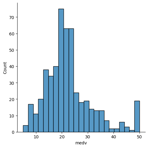
Uses, sns.displot, Seaborn to create a distribution plot (histogram) of the medv column, which represents median home values in the Boston housing dataset.
sns.displot(x=df['medv']);
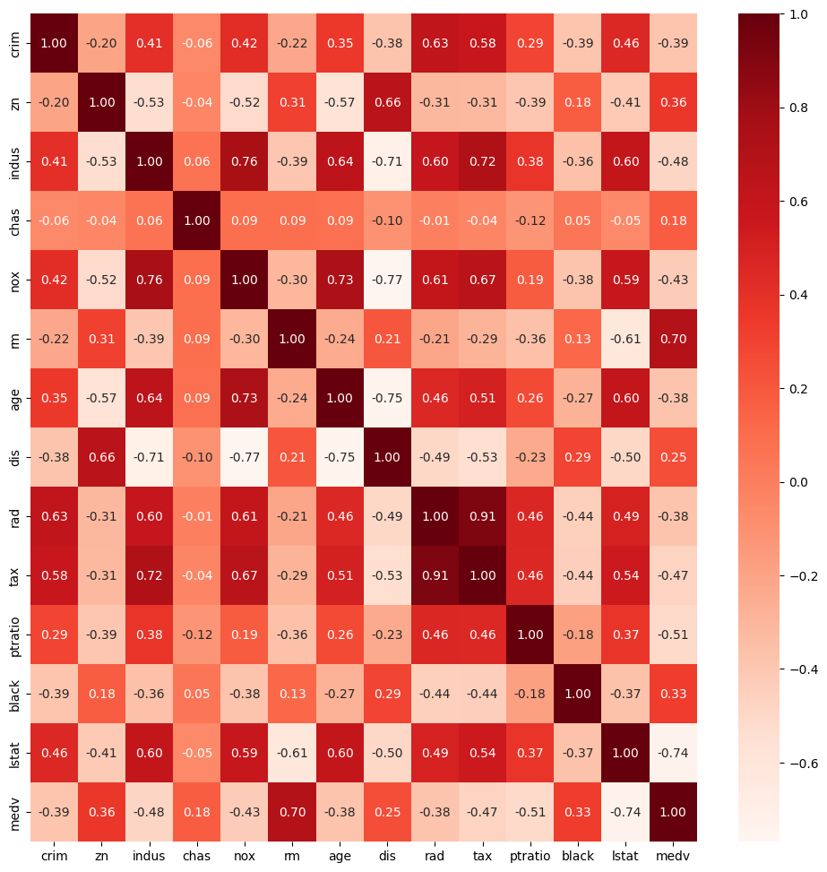
This code block creates a heatmap of the correlation matrix for the dataset df using Matplotlib and Seaborn:
What this does:
df.corr()calculates the Pearson correlation between all numeric features.sns.heatmap()visualizes this correlation matrix:Cells are color-coded by strength of correlation (red = stronger).
annot=Trueshows the numeric correlation values in each cell.fmt='.2f'ensures values are shown with 2 decimal places.
Why it’s useful:
Helps you spot strong positive or negative relationships between variables.
Useful for feature selection or identifying multicollinearity in models.
Multicollinearity occurs when two or more predictor variables are highly correlated, which can make it difficult to determine their individual effects in a regression model.
plt.figure(figsize=(12,12))
cor = df.corr()
sns.heatmap(cor, annot=True, cmap=plt.cm.Reds, fmt='.2f');
Acknowledgements#
Information, code examples, and dataset insights in this notebook were adapted or inspired by the following Kaggle resources:
Kashnitsky, A. – Topic 1: Exploratory Data Analysis with Pandas
Ziad Hamada Fathy – Boston House Price Predictions
Willian Leite – Boston Housing Dataset
Thanks to these contributors for their valuable work.
This notebook was created by Meara Cox, June 2024, as a part of her summer internship.