Pandas Intermediate 2#
Description: This notebook describes how to:
Work with time series data in Pandas
Use
.plot()to make different kinds of static charts
Use Case: For Learners (Detailed explanation, not ideal for researchers)
Difficulty: Intermediate
Knowledge Required:
Python Basics (Start Python Basics I)
Pandas Basics (Start Pandas Basics I)
Knowledge Recommended:
Completion Time: 90 minutes
Data Format: csv
Libraries Used: Pandas
Research Pipeline: None
# import Pandas, `as pd` allows us to shorten typing pandas to pd
import pandas as pd
Times series data#
Time-series data is everywhere. You see it used in public health record, weather records and many other places. Pandas library provides a comprehensive framework for working with times, dates, and time-series data.
In real life, we often find datasets where dates and times are stored as strings.
import urllib
from pathlib import Path

# Check if a data folder exists. If not, create it.
data_folder = Path('../data/')
data_folder.mkdir(exist_ok=True)

# Download the sample files
url = 'https://ithaka-labs.s3.amazonaws.com/static-files/images/tdm/tdmdocs/Pandas1_failed_banks_since_2000.csv'
file = '../data/failed_banks.csv'
urllib.request.urlretrieve(url, file)
print('Sample file ready.')

# Read in the data
banks_df = pd.read_csv(file)
banks_df
Sample file ready.
| Bank Name | City | State | Cert | Acquiring Institution | Closing Date | Fund | |
|---|---|---|---|---|---|---|---|
| 0 | First Republic Bank | San Francisco | CA | 59017 | JPMorgan Chase Bank, N.A. | 1-May-23 | 10543 |
| 1 | Signature Bank | New York | NY | 57053 | Flagstar Bank, N.A. | 12-Mar-23 | 10540 |
| 2 | Silicon Valley Bank | Santa Clara | CA | 24735 | First Citizens Bank & Trust Company | 10-Mar-23 | 10539 |
| 3 | Almena State Bank | Almena | KS | 15426 | Equity Bank | 23-Oct-20 | 10538 |
| 4 | First City Bank of Florida | Fort Walton Beach | FL | 16748 | United Fidelity Bank, fsb | 16-Oct-20 | 10537 |
| ... | ... | ... | ... | ... | ... | ... | ... |
| 561 | Superior Bank, FSB | Hinsdale | IL | 32646 | Superior Federal, FSB | 27-Jul-01 | 6004 |
| 562 | Malta National Bank | Malta | OH | 6629 | North Valley Bank | 3-May-01 | 4648 |
| 563 | First Alliance Bank & Trust Co. | Manchester | NH | 34264 | Southern New Hampshire Bank & Trust | 2-Feb-01 | 4647 |
| 564 | National State Bank of Metropolis | Metropolis | IL | 3815 | Banterra Bank of Marion | 14-Dec-00 | 4646 |
| 565 | Bank of Honolulu | Honolulu | HI | 21029 | Bank of the Orient | 13-Oct-00 | 4645 |
566 rows × 7 columns
# check the data type of the Closing Date column
banks_df['Closing Date']
0       1-May-23
1      12-Mar-23
2      10-Mar-23
3      23-Oct-20
4      16-Oct-20
         ...
561    27-Jul-01
562     3-May-01
563     2-Feb-01
564    14-Dec-00
565    13-Oct-00
Name: Closing Date, Length: 566, dtype: object
As you can see, the dates in the Closing Date column are strings. We can convert the data type to datetime using the to_datetime() function in Pandas. The strings in this column will be turned into datetime objects.
The datetime objects#
# convert the strings to datetime
banks_df['Closing Date'] = pd.to_datetime(banks_df['Closing Date'], format='%d-%b-%y')
# check the data type of the Closing Date column
banks_df['Closing Date']
0     2023-05-01
1     2023-03-12
2     2023-03-10
3     2020-10-23
4     2020-10-16
         ...
561   2001-07-27
562   2001-05-03
563   2001-02-02
564   2000-12-14
565   2000-10-13
Name: Closing Date, Length: 566, dtype: datetime64[ns]
When we parse the strings in the Closing Date column into datetime objects, we specify a format to inform Pandas of how to do the parsing. For the cheatsheet of the format codes, you can check the documentation here.
One good thing about converting the dates and times into datetime objects is that we can then use them to index a dataframe. You will soon see that indexing using datetime objects is very flexible.
# set the index to Closing Date
banks_df = banks_df.set_index('Closing Date').sort_index()
# select data between two dates
banks_df.loc['2020-01-01':'2023-07-01']
| Bank Name | City | State | Cert | Acquiring Institution | Fund | |
|---|---|---|---|---|---|---|
| Closing Date | ||||||
| 2020-02-14 | Ericson State Bank | Ericson | NE | 18265 | Farmers and Merchants Bank | 10535 |
| 2020-04-03 | The First State Bank | Barboursville | WV | 14361 | MVB Bank, Inc. | 10536 |
| 2020-10-16 | First City Bank of Florida | Fort Walton Beach | FL | 16748 | United Fidelity Bank, fsb | 10537 |
| 2020-10-23 | Almena State Bank | Almena | KS | 15426 | Equity Bank | 10538 |
| 2023-03-10 | Silicon Valley Bank | Santa Clara | CA | 24735 | First Citizens Bank & Trust Company | 10539 |
| 2023-03-12 | Signature Bank | New York | NY | 57053 | Flagstar Bank, N.A. | 10540 |
| 2023-05-01 | First Republic Bank | San Francisco | CA | 59017 | JPMorgan Chase Bank, N.A. | 10543 |
Providing the full form YYYY-MM-DD when selecting data from the dataframe is expected, as our indexes are in the format of YYYY-MM-DD. However, what makes datetime indexes really convenient is that we can do partial indexing with them!
# select data between two months
banks_df.loc['2020-01':'2023-07']
| Bank Name | City | State | Cert | Acquiring Institution | Fund | |
|---|---|---|---|---|---|---|
| Closing Date | ||||||
| 2020-02-14 | Ericson State Bank | Ericson | NE | 18265 | Farmers and Merchants Bank | 10535 |
| 2020-04-03 | The First State Bank | Barboursville | WV | 14361 | MVB Bank, Inc. | 10536 |
| 2020-10-16 | First City Bank of Florida | Fort Walton Beach | FL | 16748 | United Fidelity Bank, fsb | 10537 |
| 2020-10-23 | Almena State Bank | Almena | KS | 15426 | Equity Bank | 10538 |
| 2023-03-10 | Silicon Valley Bank | Santa Clara | CA | 24735 | First Citizens Bank & Trust Company | 10539 |
| 2023-03-12 | Signature Bank | New York | NY | 57053 | Flagstar Bank, N.A. | 10540 |
| 2023-05-01 | First Republic Bank | San Francisco | CA | 59017 | JPMorgan Chase Bank, N.A. | 10543 |
As you can see, even if we do not provide the full forms, we do not get an error.
# select data between two years
banks_df.loc['2020':'2023']
| Bank Name | City | State | Cert | Acquiring Institution | Fund | |
|---|---|---|---|---|---|---|
| Closing Date | ||||||
| 2020-02-14 | Ericson State Bank | Ericson | NE | 18265 | Farmers and Merchants Bank | 10535 |
| 2020-04-03 | The First State Bank | Barboursville | WV | 14361 | MVB Bank, Inc. | 10536 |
| 2020-10-16 | First City Bank of Florida | Fort Walton Beach | FL | 16748 | United Fidelity Bank, fsb | 10537 |
| 2020-10-23 | Almena State Bank | Almena | KS | 15426 | Equity Bank | 10538 |
| 2023-03-10 | Silicon Valley Bank | Santa Clara | CA | 24735 | First Citizens Bank & Trust Company | 10539 |
| 2023-03-12 | Signature Bank | New York | NY | 57053 | Flagstar Bank, N.A. | 10540 |
| 2023-05-01 | First Republic Bank | San Francisco | CA | 59017 | JPMorgan Chase Bank, N.A. | 10543 |
# reset the index for later use
banks_df = banks_df.reset_index()
Note that this kind of partial indexing is impossible with other data types. Let’s create a small dataframe to test what will happen if we use partial indexing with string dates.
# create a df with a column of dates stored as strings
date_str = pd.DataFrame({'Date':['2020-06-01', '2021-06-30'],
                        'num_failed_banks':[1,2]})

# set the index column to the Date column
date_str = date_str.set_index('Date')

# select data using partial indexing
date_str.loc['2020']
---------------------------------------------------------------------------
KeyError                                  Traceback (most recent call last)
File /opt/homebrew/lib/python3.11/site-packages/pandas/core/indexes/base.py:3812, in Index.get_loc(self, key)
   3811 try:
-> 3812     return self._engine.get_loc(casted_key)
   3813 except KeyError as err:

File pandas/_libs/index.pyx:167, in pandas._libs.index.IndexEngine.get_loc()

File pandas/_libs/index.pyx:196, in pandas._libs.index.IndexEngine.get_loc()

File pandas/_libs/hashtable_class_helper.pxi:7088, in pandas._libs.hashtable.PyObjectHashTable.get_item()

File pandas/_libs/hashtable_class_helper.pxi:7096, in pandas._libs.hashtable.PyObjectHashTable.get_item()

KeyError: '2020'

The above exception was the direct cause of the following exception:

KeyError                                  Traceback (most recent call last)
Cell In[12], line 9
      6 date_str = date_str.set_index('Date')
      8 # select data using partial indexing
----> 9 date_str.loc['2020']

File /opt/homebrew/lib/python3.11/site-packages/pandas/core/indexing.py:1191, in _LocationIndexer.__getitem__(self, key)
   1189 maybe_callable = com.apply_if_callable(key, self.obj)
   1190 maybe_callable = self._check_deprecated_callable_usage(key, maybe_callable)
-> 1191 return self._getitem_axis(maybe_callable, axis=axis)

File /opt/homebrew/lib/python3.11/site-packages/pandas/core/indexing.py:1431, in _LocIndexer._getitem_axis(self, key, axis)
   1429 # fall thru to straight lookup
   1430 self._validate_key(key, axis)
-> 1431 return self._get_label(key, axis=axis)

File /opt/homebrew/lib/python3.11/site-packages/pandas/core/indexing.py:1381, in _LocIndexer._get_label(self, label, axis)
   1379 def _get_label(self, label, axis: AxisInt):
   1380     # GH#5567 this will fail if the label is not present in the axis.
-> 1381     return self.obj.xs(label, axis=axis)

File /opt/homebrew/lib/python3.11/site-packages/pandas/core/generic.py:4320, in NDFrame.xs(self, key, axis, level, drop_level)
   4318             new_index = index[loc]
   4319 else:
-> 4320     loc = index.get_loc(key)
   4322     if isinstance(loc, np.ndarray):
   4323         if loc.dtype == np.bool_:

File /opt/homebrew/lib/python3.11/site-packages/pandas/core/indexes/base.py:3819, in Index.get_loc(self, key)
   3814     if isinstance(casted_key, slice) or (
   3815         isinstance(casted_key, abc.Iterable)
   3816         and any(isinstance(x, slice) for x in casted_key)
   3817     ):
   3818         raise InvalidIndexError(key)
-> 3819     raise KeyError(key) from err
   3820 except TypeError:
   3821     # If we have a listlike key, _check_indexing_error will raise
   3822     #  InvalidIndexError. Otherwise we fall through and re-raise
   3823     #  the TypeError.
   3824     self._check_indexing_error(key)

KeyError: '2020'
We got a key error! This is because ‘2020’ is not one of the indexes and partial indexing with strings is impossible. If we supply ‘2020’ as the index, Pandas will try to find the rows whose index is ‘2020’, but there are no rows with this index in our small dataframe!
The datetime class has a variety of attributes that we can access. For example, we can access the ‘year’, ‘month’, and ‘date’ from the full form of a datetime object.
# access the 'year' from datetime objects
banks_df['Closing Date'].dt.year
0      2000
1      2000
2      2001
3      2001
4      2001
       ...
561    2020
562    2020
563    2023
564    2023
565    2023
Name: Closing Date, Length: 566, dtype: int32
The datetime class also has a variety of methods that we can use. For example, if we would like to get the day of week for each date in the Closing Date column, we can use the day_name() method.
# access the day of week from datetime objects
banks_df['Closing Date'].dt.day_name()
0        Friday
1      Thursday
2        Friday
3      Thursday
4        Friday
         ...
561      Friday
562      Friday
563      Friday
564      Sunday
565      Monday
Name: Closing Date, Length: 566, dtype: object
The attributes and methods available in the datetime class make it extremely easy to extract the ‘year’, ‘month’ and ‘date’ into different columns.
In the following code cell, can you write some code to create a new column that contains the closing years of the banks? In Pandas basics 2, we did it with string slicing, but this time let’s try using the attributes of the datetime class to do it.
# create a new column containing the closing years
Grouping data using the datetime objects is also quite convenient. We can use the resample() method to specify the granularity with which we would like to group the data.
# group the data using resample()
banks_df.resample('Y', on='Closing Date').size()
/var/folders/2h/84wxzls579b1yv00g4jj02fh0000gn/T/ipykernel_21161/312667976.py:2: FutureWarning: 'Y' is deprecated and will be removed in a future version, please use 'YE' instead.
  banks_df.resample('Y', on='Closing Date').size()
Closing Date
2000-12-31      2
2001-12-31      4
2002-12-31     11
2003-12-31      3
2004-12-31      4
2005-12-31      0
2006-12-31      0
2007-12-31      3
2008-12-31     25
2009-12-31    140
2010-12-31    157
2011-12-31     92
2012-12-31     51
2013-12-31     24
2014-12-31     18
2015-12-31      8
2016-12-31      5
2017-12-31      8
2018-12-31      0
2019-12-31      4
2020-12-31      4
2021-12-31      0
2022-12-31      0
2023-12-31      3
Freq: YE-DEC, dtype: int64
With resample(), we can choose to upsample or downsample.
# downsample to month with smaller granularity
banks_df.resample('M', on='Closing Date').size()
/var/folders/2h/84wxzls579b1yv00g4jj02fh0000gn/T/ipykernel_21161/3076179390.py:2: FutureWarning: 'M' is deprecated and will be removed in a future version, please use 'ME' instead.
  banks_df.resample('M', on='Closing Date').size()
Closing Date
2000-10-31    1
2000-11-30    0
2000-12-31    1
2001-01-31    0
2001-02-28    1
             ..
2023-01-31    0
2023-02-28    0
2023-03-31    2
2023-04-30    0
2023-05-31    1
Freq: ME, Length: 272, dtype: int64
# upsample to 12 hours with greater granularity
banks_df.resample('12H', on='Closing Date').size()
/var/folders/2h/84wxzls579b1yv00g4jj02fh0000gn/T/ipykernel_21161/2767640105.py:2: FutureWarning: 'H' is deprecated and will be removed in a future version, please use 'h' instead.
  banks_df.resample('12H', on='Closing Date').size()
Closing Date
2000-10-13 00:00:00    1
2000-10-13 12:00:00    0
2000-10-14 00:00:00    0
2000-10-14 12:00:00    0
2000-10-15 00:00:00    0
                      ..
2023-04-29 00:00:00    0
2023-04-29 12:00:00    0
2023-04-30 00:00:00    0
2023-04-30 12:00:00    0
2023-05-01 00:00:00    1
Freq: 12h, Length: 16471, dtype: int64
In Pandas intermediate 1, you have learned how to group the data using groupby(). In the next code cell, can you use both groupby() and resample() to get how many banks were failed in each state by year?
# get how many banks were failed in each state by year
The timedelta objects#
In Pandas, the difference between two time points is a timedelta object. In other words, while datetime objects are used to represent instants of time, timedelta objects are used to represent durations of time.
When you substract one datetime object from another, you’ll get a timedelta object.
# substract one time point from another
pd.to_datetime('2020-06-01 12:00:00') - pd.to_datetime('2020-06-01 8:00:00')
Timedelta('0 days 04:00:00')
In the following, let’s grab the 2022 Boston Marathon dataset and use the completion time of the runners as an example.
# Get the urls to the files and download the files
import urllib.request
url = 'https://ithaka-labs.s3.amazonaws.com/static-files/images/tdm/tdmdocs/DataViz3_BostonMarathon2022.csv'
urllib.request.urlretrieve(url, '../data/'+url.rsplit('/')[-1][9:])

# Success message
print('Sample file ready.')

# create a dataframe
bm_22 = pd.read_csv('../data/BostonMarathon2022.csv')

# get the data type of the OfficialTime column
bm_22['OfficialTime'].info()
Sample file ready.
<class 'pandas.core.series.Series'>
RangeIndex: 24834 entries, 0 to 24833
Series name: OfficialTime
Non-Null Count  Dtype
--------------  -----
24834 non-null  object
dtypes: object(1)
memory usage: 194.1+ KB
# turn the data type of the OfficialTime column to timedelta
bm_22['OfficialTime'] = pd.to_timedelta(bm_22['OfficialTime'])
# get the difference in completion time between the
# fastest runner and the slowest runner
bm_22['OfficialTime'].max() - bm_22['OfficialTime'].min()
Timedelta('0 days 05:17:48')
Just like the datetime objects, the timedelta objects also have a variety of attributes and methods that we can make use of.
# get the components of a timedelta object
bm_22['OfficialTime'].dt.components
| days | hours | minutes | seconds | milliseconds | microseconds | nanoseconds | |
|---|---|---|---|---|---|---|---|
| 0 | 0 | 2 | 6 | 51 | 0 | 0 | 0 |
| 1 | 0 | 2 | 7 | 21 | 0 | 0 | 0 |
| 2 | 0 | 2 | 7 | 27 | 0 | 0 | 0 |
| 3 | 0 | 2 | 7 | 53 | 0 | 0 | 0 |
| 4 | 0 | 2 | 8 | 47 | 0 | 0 | 0 |
| ... | ... | ... | ... | ... | ... | ... | ... |
| 24829 | 0 | 6 | 56 | 35 | 0 | 0 | 0 |
| 24830 | 0 | 6 | 58 | 12 | 0 | 0 | 0 |
| 24831 | 0 | 6 | 58 | 50 | 0 | 0 | 0 |
| 24832 | 0 | 7 | 1 | 32 | 0 | 0 | 0 |
| 24833 | 0 | 7 | 24 | 39 | 0 | 0 | 0 |
24834 rows × 7 columns
# Get the completion time in seconds
bm_22['OfficialTime'].dt.total_seconds()
0         7611.0
1         7641.0
2         7647.0
3         7673.0
4         7727.0
          ...
24829    24995.0
24830    25092.0
24831    25130.0
24832    25292.0
24833    26679.0
Name: OfficialTime, Length: 24834, dtype: float64
Suppose you would like to get the average completion time of the runners in the United States. How do you do that?
# get the average completion time of the runners in the US
Plotting in Pandas#
Pandas uses the .plot() method to create charts and plots. In this section, we’ll learn how to use the .plot() method to make different kinds of charts.
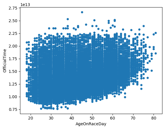
Scatterplot#
Scatter plots are usually used to show the relationship between different variables. Suppose we would like to see whether there is a relationship between the age of the runners and their completion time.
# prepare the data
bm_22_sc = bm_22[['AgeOnRaceDay', 'OfficialTime']].copy()

# make a scatter plot
bm_22_sc.plot(kind='scatter', x='AgeOnRaceDay', y='OfficialTime')
<Axes: xlabel='AgeOnRaceDay', ylabel='OfficialTime'>
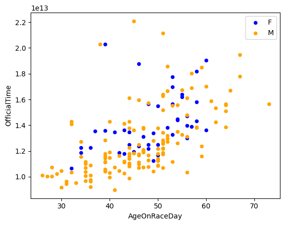
If the data are categorically grouped, you can slice the data into smaller data series and color them differently.
For example, suppose we are interested in the relationship between the age and the completion time of the runners from France.
# prepare the data
bm_22_sc_fm = bm_22.loc[bm_22['CountryOfResName']=='France'][['AgeOnRaceDay', 'OfficialTime', 'Gender']].copy()
bm_22_sc_fm = bm_22_sc_fm.sort_values(by='Gender').reset_index(drop=True)

# get the cutting point in the Gender column
bm_22_sc_fm.loc[bm_22_sc_fm['Gender']=='F'].tail(1)
| AgeOnRaceDay | OfficialTime | Gender | |
|---|---|---|---|
| 42 | 58 | 0 days 04:23:33 | F |
# make a scatter plot
ax1 = bm_22_sc_fm.loc[:42].plot(kind='scatter',
                                   x='AgeOnRaceDay',
                                   y='OfficialTime',
                                   c='blue',label='F')

ax2 = bm_22_sc_fm.loc[43:].plot(kind='scatter',
                                   x='AgeOnRaceDay',
                                   y='OfficialTime',
                                   c='orange',label='M', ax=ax1)
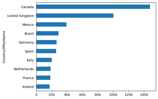
Bar charts#
In Pandas intermediate 1, we have plotted a bar chart showing the number of failed banks by year in the failed banks dataset. In this section, let’s plot more kinds of bar charts. Suppose we would like to get the top ten non-US countries with the most runners and plot the number of runners from them in a horizontal bar chart.
# prepare the data
bm_22_hbar = bm_22.groupby('CountryOfResName').size().sort_values().iloc[-11:-1]
bm_22_hbar
CountryOfResName
Ireland            172
France             183
Netherlands        185
Italy              202
Spain              258
Germany            264
Brazil             288
Mexico             393
United Kingdom    1002
Canada            1478
dtype: int64
# make a horizontal bar chart
bm_22_hbar.plot(kind='barh')
<Axes: ylabel='CountryOfResName'>
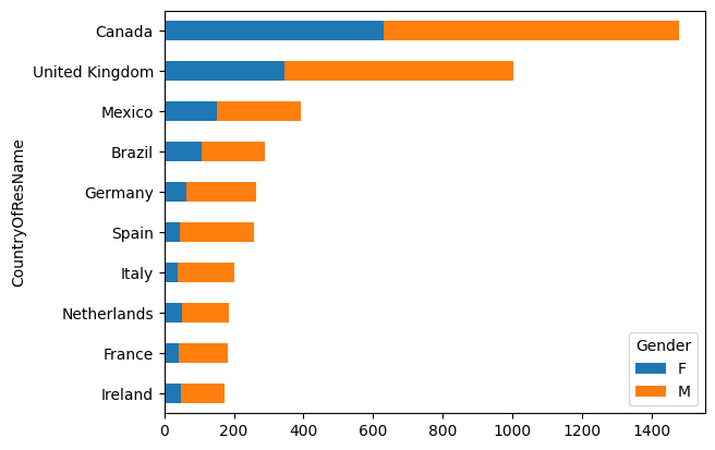
Now, suppose we would like to break the total number of runners in each country by gender and make a stacked bar chart instead.
# prepare the data
bm_22_sthbar = bm_22[['CountryOfResName', 'Gender']].copy()

# get the names of the top 10 non-US countries with the most runners
ctry = bm_22_sthbar.groupby('CountryOfResName').size().sort_values().iloc[-11:-1].index

# restructure the df for plotting
bm_22_sthbar = bm_22_sthbar.loc[bm_22_sthbar['CountryOfResName'].isin(ctry)].copy()
bm_22_sthbar = bm_22_sthbar.groupby(['CountryOfResName', 'Gender']).size().to_frame().unstack()
bm_22_sthbar.columns = bm_22_sthbar.columns.droplevel(0)
bm_22_sthbar['sum'] = bm_22_sthbar['F'] + bm_22_sthbar['M']
bm_22_sthbar = bm_22_sthbar.sort_values(by='sum').drop(columns='sum')
# make the stacked horizontal bar chart
bm_22_sthbar.plot(kind='barh', stacked=True)
<Axes: ylabel='CountryOfResName'>
Coding Challenge! < / >
Can you plot another bar chart showing the number of female and male runners from the same ten countries but this time with the two bars for each country standing next to each other?
# make a bar chart showing the number of female and male runners
# of the top non-US countries with the most runners
# with two bars for each country, one for female, one for male
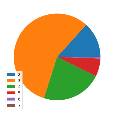
Pie chart#
A pie chart is usually used to show how a total amount is divided between different levels of a categorical variable. In a pie chart, the levels of a categorical variable is represented by a slice of the pie.
Let’s make a pie chart that shows how the total number of runners are divided between the completion time in hours.
### prepare the data

# get the column(s) of interest
bm_22_pie = bm_22[['OfficialTime']].copy()

# create a new column containing the hours
bm_22_pie['Hour'] = bm_22_pie['OfficialTime'].dt.components['hours']

# group the data by Hour and get how many runners there are in each subgroup
bm_22_pie = bm_22_pie.groupby('Hour').size()

# make the pie chart
bm_22_pie.plot(kind='pie', labels=None, legend=True)
<Axes: >
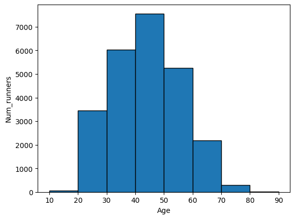
Histogram#
A histogram is a bar chart which shows the frequency of observations. In a histogram, the x-axis is a continuous quantitative value. The height of each bar shows the frequency of a certain range of values. The biggest difference between a bar chart and a histogram is that a bar chart has categorical values on the x-axis but a histogram has continuous quantitative values on the x-axis.
Suppose we are interested in the distribution of the age of the runners in ranges of 10. How many runners were of age 20 - 29 at the time of race? How many were of age 30 - 39? Moreover, we would like to make a histogram that shows the distribution of age. Before we do that, can you take a guess which age group has the most runners?
# get the youngest and oldest age
print(bm_22['AgeOnRaceDay'].max())
print(bm_22['AgeOnRaceDay'].min())
81
18
# prepare the data for plotting
bm_22_hist = bm_22['AgeOnRaceDay'].copy()

# make a range of bins
bins = range(10, 100, 10)

bm_22_hist.plot(kind='hist', bins=bins, edgecolor='black', xlabel='Age',ylabel='Num_runners')
<Axes: xlabel='Age', ylabel='Num_runners'>
In the next code cell, can you make a histogram that displays the distribution of the completion time of the runners in ranges of 1 hour?
# make a histogram displaying the distribution of
# the completion time of the runners in ranges of 1 hour
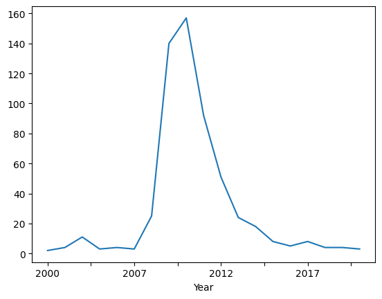
Line graph#
A line graph consists of points connected by line segments. It is commonly used to demonstrate changes in value. Oftentimes, the horizontal axis holds “time” and the vertical axis shows the change in a value of interest.
In Pandas intermediate 1, we made a bar chart to display the number of failed banks by year. Let’s make a line graph to show the change in the number over the years in that dataset.
### prepare the data for plotting

# get the column(s) of interest
banks_line = banks_df[['Closing Date']].copy()

# create a new column containing the years
banks_line['Year'] = banks_line['Closing Date'].dt.year.astype(str)

# group the data by year and get how many banks failed in each year
banks_line = banks_line.groupby('Year').size()

# plot the line graph
banks_line.plot(xlabel='Year')
<Axes: xlabel='Year'>
Lesson Complete#
Congratulations! You have completed Pandas Intermediate 2.
Start Next Lesson: Pandas intermediate 3 ->#
Exercise Solutions#
Here are a few solutions for exercises in this lesson.
# get how many banks were failed in each state by year
banks_df.groupby('State').resample('Y', on='Closing Date').size()
# get the average completion time of the runners from the US

# Get the url to the file and download the file
import urllib.request
url = 'https://ithaka-labs.s3.amazonaws.com/static-files/images/tdm/tdmdocs/DataViz3_BostonMarathon2022.csv'
urllib.request.urlretrieve(url, '../data/'+url.rsplit('/')[-1][9:])

# Success message
print('Sample file ready.')

# create a dataframe
bm_22 = pd.read_csv('../data/BostonMarathon2022.csv')

# turn the 'OfficialTime' column to type timedelta
bm_22['OfficialTime'] = pd.to_timedelta(bm_22['OfficialTime'])

# get the average completion time of the runners in the US
bm_22.loc[bm_22['CountryOfResName']=='United States of America']['OfficialTime'].mean()
## create a bar chart with two bard next to each other for each country
# prepare the data
bm_22_bar_fm = bm_22[['CountryOfResName', 'Gender']].copy()

# get the names of the top 10 non-US countries with the most runners
ctry = bm_22_bar_fm.groupby('CountryOfResName').size().sort_values().iloc[-11:-1].index

# restructure the df for plotting
bm_22_bar_fm = bm_22_bar_fm.loc[bm_22_bar_fm['CountryOfResName'].isin(ctry)].copy()
bm_22_bar_fm = bm_22_bar_fm.groupby(['CountryOfResName', 'Gender']).size().to_frame().unstack()
bm_22_bar_fm.columns = bm_22_bar_fm.columns.droplevel(0)

# plot the bar chart
bm_22_bar_fm.plot(kind='bar')
### make a histogram showing the distribution of completion time
### in ranges of 1 hour

# Get the url to the file and download the file
import urllib.request
url = 'https://ithaka-labs.s3.amazonaws.com/static-files/images/tdm/tdmdocs/DataViz3_BostonMarathon2022.csv'
urllib.request.urlretrieve(url, '../data/'+url.rsplit('/')[-1][9:])

# Success message
print('Sample file ready.')

# create a dataframe
bm_22 = pd.read_csv('../data/BostonMarathon2022.csv')

# get the column of interest
bm_22_time = bm_22[['OfficialTime']].copy()

# make a new column containing the hour only
bm_22_time['Hour'] = bm_22_time['OfficialTime'].str[0].astype(int)

# get the max and min value from OfficialTime
min_h = bm_22_time['Hour'].min()
max_h = bm_22_time['Hour'].max()

# make the bins
bins = range(min_h, max_h+2)

# plot the histogram
bm_22_time['Hour'].plot(kind='hist', logy=True, bins=bins, edgecolor='black', ylabel='Num_runners')